A Simple Network Analysis

In this section of Introduction to Network Analysis in R. I assume that we have imported and have a basic graph object. Now we want to explore the network and see what we have.

The R-data file for this section: campnet.rda.

The R-script for this section (with some bonus features, I think): simpleNetworkAnalysis.R

Here is what I cover here:

1. Filtering the network
2. Centrality and power
3. Local position
4. Whole network stats
5. Putting everything together
6. Extracting the results

Filtering the network

I start with the assumption that have the network g which has edges for both time-points present in the graph object.

1. Only keep edges with a weight less than four. (this network uses ranking for weight meaning 1, 2, 3 are the three strongest weights, larger numbers are weaker)
2. Create two networks at each time point

# filter the network for only the top three picks
g.edge3 <- subgraph.edges(g, which(E(g)$weight < 4))

# time 1 and 2
g1.edge3 <- subgraph.edges(g.edge3, which(E(g.edge3)$time == 1))
g2.edge3 <- subgraph.edges(g.edge3, which(E(g.edge3)$time == 2))

We can actually put both the time points into a single object so we can easily loop over all the time points when doing analysis.

# stack both time points into a list
gs <- list()
gs[[1]] <- g1.edge3
gs[[2]] <- g2.edge3

Now we can access each time point using the list instead of the g1.edge3 object directly. This seems convoluted, but if you have many (dozens, hundreds, thousands) of different networks to analyze a list of graph objects can be very useful. We will analyze the graphs using the lapply function. When we move to high performance computing, it becomes trivial to do multi-core processing using mcapply if you get used to using lapply first.

Note, I’m also renaming / removing the weight attribute. Many of the functions will use a weight attribute if it exists by default. Since we have already filtered on weight, it’s no longer important. We can safely assume that the network is just a directed, un-weighted network. Also the function incorrectly assume that a higher value for weight is a stronger connection, but it’s the opposite for our data. I’m going to reverse the direction (subtract the value from the max value and add one).

# renaming and reversing the weight attribute and
E(g.edge3)$wt <- max(E(g.edge3)$weight) - E(g.edge3)$weight + 1
remove.edge.attribute(g.edge3, 'weight')

Centrality and Power Measures

Node centrality is a property of a position in a network. It can indicate how powerful the position is, how likely this position is to intercept information, how easy it is for a node in the position to control information, etc. I tend to categorize centrality measures in four ways, activity, control, efficiency, and total effects.

• Activity - how active a node is in the network
• Control - how much control a node can exert
• Efficiency - how close a node is to every other node in the network
• Total Effects - where a node’s centrality is a function of the centrality of others
• Other - in this case, we will look at edge-properties

Each time we caculate an centrality we are going to add it to the graph object as an attrbute. That way we can keep all results of our analyses in one place.

Activity: Degree

Degree is a way of measuring node activity. There are a few ways of measuring degree.

• Total-degree is the count of all edges incident (connected to) a node
• In-degree is the count of all edges that point in to a node
• Out-degree is the count of all edges that point out of a node

# the default is total degree
degree(g1.edge3)
degree(g1.edge3, mode = 'total')
degree(g1.edge3, mode = 'in')
degree(g1.edge3, mode = 'out')

Control: Betweenness

Betweenness is a way of measuring node control. Betweenness is calculated for each node by looking at the number of shortest paths between every pair of nodes in the network and counting how many of those paths goes through the subject node. Betweenness behaves strangely with weigthed / valued networks because the shortest paths can be skewed or reduced dramatically. In some cases this makes sense, but it’s important to understand that only the shortest paths are considered.

Withought a weight variable on your edges, betweenness is a very simple line of code.

betweenness(g1.edge3)

If you want to use weights in such a way that you are measuring flow of information you will want to consider flow betweenness. The igraph package does not have an implementation of flow betweenness, but the sna package does. I don’t recommend loading both igraph and sna at the same time since many of the function names will conflict with each other and cause errors. Intead use the double-colon package operator :: to directly access functions in other packages without loading them completely. The package has to be installed at least.

# get a numeric adjacency matrix of the network where the entries are the weights of the ties
mat <- as.matrix(get.adjacency(g1.edge3, attr = "wt"))
# calculate flow betweenness
sna::flowbet(mat)

Effeciency: Closeness

Closeness is a way of measuring node efficiency. It is a measure of how close on average a node is to every other node in the network.

closeness(g1.edge3)

Overall: Eigenvector

Eigenvector centrality is a way of measuring the total effects centrality of a node position. The evcent function doesn’t just output the centrality measures, it returns a list with the measures and all the other attributes of the calculation. If you just want the centrality and nothing else you just access the vector data.

evcent(g1.edge3)$vector

Other: Edge Betweenness

Edge betweenness measures the centrality or control of an edge in the network. It can be a measure of how important a single relationship is between two nodes. The edges with high betweenness

edge.betweenness(g1.edge3)

The lapply function takes a list and applies a function to each element of the list. In this case each element is a graph object. It’s passed to a function, in this case an anonymous function, as x. So then each centrality measure is calculated and stored into x and then x is returned. You give lapply a list and it will return a list.

Local Position

The centrality measures use network paths to calculate power and influence. That is they trade paths through the network where a node is visited only once. Except for degree, which I think should really be a local position measure, but it’s nearly always thought of as a centrality measure.

Local position considers just the immediate neighborhood around a node and how that influences power and independence.

Effective size

A person may have 10 ties to people, but if 5 of those ties go out to a group that all have ties with each other, and the other 5 ties go to a group that are also connected, then the focal person (or ego) has a network with lots of redundancy. Effective size is the size of an ego’s network minus that redundancy. You can read more about it here.

This is an example of where neither igraph or sna have the function for measuring effective size. It’s also a great of example how to use Stack Overflow for help. If you Google “stack overflow igraph effective size” your first link is the answer to your question. Someone has provided a function that will calculate effective size for a given node. The elipses ... allow us to pass a number of arbitrary arguments to neighbors if we want. Which is important since this is a directed network. Thanks to Ofrit Lesser for some bug fixes on this code.

# definite a function like this
ego.effective.size <- function(g, ego, ...) {
  egonet <- induced.subgraph(g, neighbors(g, ego, ...))
  n <- vcount(egonet)
  t <- ecount(egonet)
  return(n - (2 * t) / n)
}
# then call it like this
ego.effective.size(g1.edge3, "BRAZEY")

The function takes a graph object and a node name. It finds the list of neighbors of the node (ego). Then it counts all the edges that the neighbors have that are not connected to ego. Then it counts the number of neighbors. Then uses Borgatti’s re-formulation of effective size. Notably it only calculates it for a single node.

Here is my expansion on this function. The ego=NULL line in the new function sets a default value. Below you can see that if ego is not null it will do the original ego.effective.size, but if it is null it will use sapply to apply the function to each time in the graph object and return the result.

effective.size <- function(g, ego=NULL, ...) {
  if(!is.null(ego)) {
    return(ego.effective.size(g, ego, ...))
  }
  return (sapply(V(g), function(x) {ego.effective.size(g,x, ...)}))
}
effective.size(g, mode='all')

Constraint

A structural hole is a simple case of a person knowing two other people who don’t know each other. One way to measure this is with constraint. Constraint is a measure of how much the other people know each other. That is, if your mother is close friends with your boyfriend then it becomes difficult to get away with, um, exciting activities, right? Your behavior is constrained because your contacts know each other and could possibly share information. Constraint is roughly the inverse of structural holes. It can be applied to weighted networks as well, but for now we will focus on the binary case.

constraint(g1.edge3)

Whole Network

Whole network statistics tell you about the global properties of the network.

Network size

The number of nodes in a network. The number of edges in a network.

vcount(g1.edge3)
ecount(g1.edge3)

Components

Not every network is completely connected. There could be isolates, or groups of nodes connected to each other but not the rest of the network. We call those parts of the network components and the largest component is the giant component. Our network is just a single component, but if you had multiple components you use the clusters function to test and extract them.

# Note: not run
# extract the components
g.components <- clusters(g)

# which is the largest component
ix <- which.max(g.components$csize)

# get the subgraph correspondent to just the giant component
g.giant <- induced.subgraph(g, which(g.components$membership == ix))

Density

This the number of edges in a network divided by the total number of possible edges. Note that density is not an igraph function.

graph.density(g1.edge3)

Average Path Length

How long are the paths around the network on average?

average.path.length(g1.edge3)

Centralization

Centralization is the extent to which the centrality of the network is concentrated in only a few nodes. If centrality is more evenly distributed this number will be low. If you have a network like a spoked wheel it will be very high. Any centrality measure can have a centralization score applied to it. There are many pre-built centralization functions in igraph - here are the two I tend to use.

centralization.betweenness(g1.edge3)$centralization
centralization.degree(g1.edge3)$centralization

Clusters and Cohesion

I wasn’t sure where to put clustering. If you want a very good review of clustering or community detection in graphs / networks, check out Fortunato 2010 here he has a nice book-length treatise on the topic. An entire class of algorithms focus on maximizing a value called modularity - which is a sort of p-value for clusters in networks. It asks are nodes connected within their clusters (modules) more than between clusters than they would by chance?

For now, let’s use the Girvan-Newman method to find some clusters in our network. See the animation, linked below. It calulates the edge betweenness of the network, removes the edge with the highest betweenness, checks to see if it broke the network into components, if it broke then it calculates modularity. It keeps doing this until modularity starts to decrease. It works on the assumption that edges with high betweenness are bridging communities together.

com <- edge.betweenness.community(g1.edge3)

The cluster assignments are found in a membership vector. Do not assign this value to a vertex property called membership that attribute is reserved. It will mess up different aspects of your analysis and visualization. Just assign it to something like m or memb as I’ve done here.

V(g1.edge3)$memb <- com$membership

And finally you can get the whole network property modularity, technically optimized modularity. Finding the actual maximum modularity for a graph is NP-complete so as to be impossible for even reasonably small networks.

modularity(com)

You can do a nice plot of the clusters using convex hulls easily:

com <- edge.betweenness.community(g1.edge3)
plot(com, g1.edge3)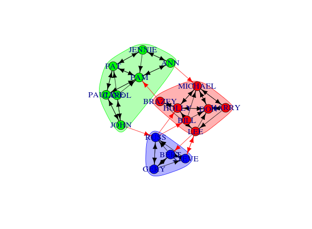

Putting it all together

As I mentioned, both time points are different graph objects in a list. This way we can process them using lapply. This code will take each graph object calculate the centrality and add it to the graph object, then return the graph object back. If you had hundreds of networks / graphs to calculate statistics on, you could process them all in one block of simple code like this. This way if you had to make changes to the analysis, you could make the change in one place and re-run all the analyses in a single burst.

gs <- lapply(gs, function(x) {
  # Centrality
  V(x)$degree      <- degree(x, mode = "total")
  V(x)$indegree    <- degree(x, mode = "in")
  V(x)$outdegree   <- degree(x, mode = "out")
  V(x)$betweenness <- betweenness(x)
  V(x)$evcent      <- evcent(x)$vector
  V(x)$closeness   <- closeness(x)
  V(x)$flowbet     <- sna::flowbet(as.matrix(get.adjacency(x, attr="wt")))
  E(x)$betweenness <- edge.betweenness(x)
  
  # Local position
  V(x)$effsize     <- effective.size(x, mode = "all")
  V(x)$constraint  <- constraint(x)
  
  # Clustering
  com <- edge.betweenness.community(x)
  V(x)$memb        <- com$membership
  
  # Whole network
  set.graph.attribute(x, "density", graph.density(x))
  set.graph.attribute(x, "avgpathlength", average.path.length(x))
  set.graph.attribute(x, "modularity", modularity(com))
  set.graph.attribute(x, "betcentralization", centralization.betweenness(x)$centralization)
  set.graph.attribute(x, "degcentralization", centralization.degree(x, mode = "total")$centralization)
  set.graph.attribute(x, "size", vcount(x))
  set.graph.attribute(x, "edgecount", ecount(x))
    
  return(x)
})

Extracting Results for Other Purposes

If you want to get your data out of the graph object for analyses use the get.data.frame function.

get.data.frame(g1.edge3, what = "vertices")
get.data.frame(g1.edge3, what = "edges")

For our list of graphs (two in this case, but easily extended) we can pull each out and add a “time” id variable using lapply and do.call('rbind', ...).

vstats <- do.call('rbind', lapply(1:length(gs), function(x) {
  o <- get.data.frame(gs[[x]], what = 'vertices')
  o$time <- x
  return(o)
}))

estats <- do.call('rbind', lapply(1:length(gs), function(x) {
  o <- get.data.frame(gs[[x]], what = 'edges')
  return(o)
}))

For the whole network level statistics, there is not a useful command like get.data.frame. Instead of we have to pull the list of attribute names and extract them one by one. In this case I use sapply to loop over the attrbute names and pull them out and return a vector. Then I use lapply to do this for each graph in the list object.

gstats <- do.call('rbind', lapply(gs, function(y) {
  ga <- list.graph.attributes(y)
  sapply(ga, function(x) {
    get.graph.attribute(y, x)
  })
}))

There. Now you have a set of data tables all ready to be merged into your other survey or observational data so you can test some hypotheses or show off to clients. Whee!